
vlookup
查找并在表中检索信息
vlookup函数是“垂直查找”的首字母缩写词,是最必不可少的工具之一Excel. It lets you look up and retrieve information stored in a table based on the value of an item in another cell.
vlookupis especially useful when you have data stored in two different tables related to each other. With this function, you can combine data from both tables into one easily readable format. Let's take a closer look at how VLOOKUP works.

What is the VLOOKUP Function in excel?
Vlookup是一个函数,可让您查找具有垂直组织表中另一个单元格中项目值的数据。要使用vlookup,请在表中的其中一列中输入您要查找的项目,然后该功能从您喜欢的任何行中返回信息与该项目相对应。
例如,我们提供了XYZ Inc.的以下员工数据。

If we intend to determine Daniel's salary, we can use the VLOOKUP function, enter "Daniel" into our formula, select the range, and VLOOKUP would return the salary as $188,000.
vlookup公式
Vlookup函数是一个简单的公式,它根据公式中的参数返回值。
The syntax for VLOOKUP is given by:
=VLOOKUP(lookup_value,table_array,column_index_num,[range_lookup])
where,
lookup_value= The value to look for in the beginning of the table i.e first column value
table_array= the table from which the value is to be retrieved
column_index_num= this parameter intends to retrieve value from our expected column
range_lookup= Optional parameter. TRUE gives an approximate match if exact match is not found, and FALSE gives an exact match or will return an error if an exact match is not found
Vookup语法的简单版本可以以下方式给出:
= vlookup(您要查找的值,您要查找的值的范围,所选值的列列,近似匹配(true)或精确匹配(false))
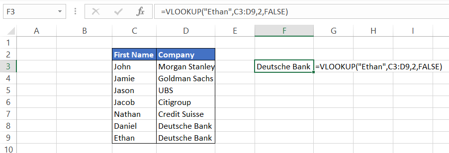
例如,我们需要找到“ Ethan”工作的投资银行。然后,我们可以使用vlookup函数,该函数将返回值为“Deutsche Bank“我们的结果,因为它出现在列Drow 9 of the table.
how to use VLOOKUP in Excel
The VLOOKUP function is pretty straightforward to use. First, you'll need to provide an example of the data you're looking for and the table in which it's stored. The VLOOKUP function will then search the left-hand column in the table for a value that matches your search criteria and return a corresponding value from the same row.
STEP 1: Arrange your data from left to right
vlookupcan only find values to the right of the column being looked up, so if yourlookup_value是在表末端或在表之间,它将无法检索值并给您错误。相反,安排数据,以便lookup_valueis to the left, and all the corresponding information you need to retrieve is on the right side of thelookup_valueto avoid getting the #N/A error.

步骤2:确定lookup_value
lookup_valuedefines what the user is looking for. Excel is highly flexible and can look up names, numbers, and even dates. For example, in this case, ourlookup_value列表在列B中。
STEP 3: Define thetable_array
Thetable_arrayargument guides VLOOKUP where to find thelookup_valueand, if found, what value to return from the selected range or table. You can choose thetable_arrayfrom the same spreadsheet, a different spreadsheet, or even an entirely different workbook. In our example, thetable_arrayis B5:E12.
STEP 4:column_index_num
Thecolumn_index_numacts as a constraint and specifies the column from which we want to retrieve the value. These are defined by numbers rather than alphabets in our formula. The VLOOKUP function cannot determine the column number by itself from which we want to retrieve the value, and hence the user needs to define the number in the formula. Ourtable_array有四列,column_index_numcan be either 1, 2, 3, or 4. (Using thecolumn_index_num因为1没有道理,也没有为用户提供太多价值。)
Note:您将收到#Value!错误,如果是column_index_num小于1。
步骤5:在精确和近似值之间选择
This is an optional yet the most crucial parameter of the VLOOKUP function. It commands Excel to find an exact or an approximate match for thelookup_value. The default value is always TRUE (1) if you don't mention or skip the argument. However, by using the FALSE (0), you can get an exact match for the data and avoid all the wrong results while looking for data.
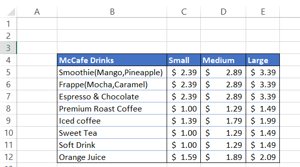
For example, let's say we want to find the price of medium-sized Iced Coffee from the McDonald's menu. To do this, type the formula=VLOOKUP(G5, B4:E12, 3, FALSE)
In "McCafe Drinks," we have a list of products with corresponding prices for small, medium, and large-sized drinks. We have referenced cell G5 to receive the price for different items on the menu dynamically.
在这种情况下,中型冰咖啡的价格为$ 1.79。同样,如果我们想找到大型冰咖啡的价格,我们只需要更改column_index_numto the column from which we expect our value. Here, we change ourcolumn_index_num通过将我们的公式更改为3到4=VLOOKUP(G5, B4:E12, 3, FALSE).


何时以及为什么使用vlookup
vlookupis commonly used intwo scenarios:
- When you're looking for a value in a table and know in which column the value exists. For example, suppose if you have a list of customers with their contact information and know that customers' age is given in column D. By specifying the column number, you can retrieve the age of the customers.
- To check whether a particular value exists in our data table. For example, if you are looking for the address of the employees in your database based on Full Name and the result gives you the #N/A error, it means that the address for the employee does not exist in your database.
vlookup允许您在两种情况下指定要查找或返回的值。这称为“查找值”。您还需要提供有关查找值的其他信息,包括它在哪个列以及在哪个表中。要执行此操作,只需输入=VLOOKUP(lookup_value,table_array), 在哪里lookup_valueis the value that links to your data set, andtable_arrayis the name of the table that contains that data set.
vlookupin financial modeling and financial analysis
建立财务模型时, you want toforecastwhat will happen in the future as accurately as possible. To do this, you need a lot of data from the past.
To forecast your future financial situation, you need to understand how the present conditions will affect the future. For example, if you are working on yourincome statement modelpredicting revenues in the upcoming years, how will it更改您的净收入and每股收益?
创建这些模型时,Vlookup函数至关重要,因为它使您可以通过将其与当前数据链接到模型中。
假设您已经对您的收入增长驱动力进行了假设表financial model. If your current annual revenue is $42,051 million and today's date is December 15th, 2021, Excel pulls up an expected value for December 15th, 2022 of $45,205 million based on the revenue growth driver using the VLOOKUP function. You don't have to calculate this yourself!
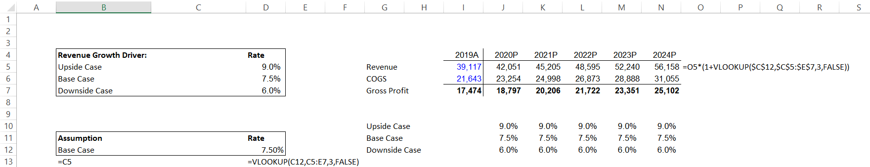
In the example above, we use the formula=O5*(1 + VLOOKUP($C$12, $C$5:$E$7, 3, FALSE))to pull in the data from revenue growth driver assumptions in cells J5:N5. By simply changing the value in cell C5 to either upside case or downside case, our financial model will reflect the revenue based on a 9% rate for upside case or a 6% rate for downside case.
Vlookup的优势
- 两种匹配模式: Based on the selection of optional parameters TRUE or FALSE, the user can find either an approximate match or an exact match, respectively, based on the user preference.
- 便于使用: It is relatively easier to use once you get the hang of it as syntax components are straightforward.
- 节省时间:通过使用vlookup,用户可以节省通常花费的时间手动查找数据或任何其他类似的任务。
Limitations of VLOOKUP
- vlookupalways looks right: It means that your data must be oriented from left to right with yourlookup_valueat the extreme left. The function will not work if you intend to retrieve values to your left.
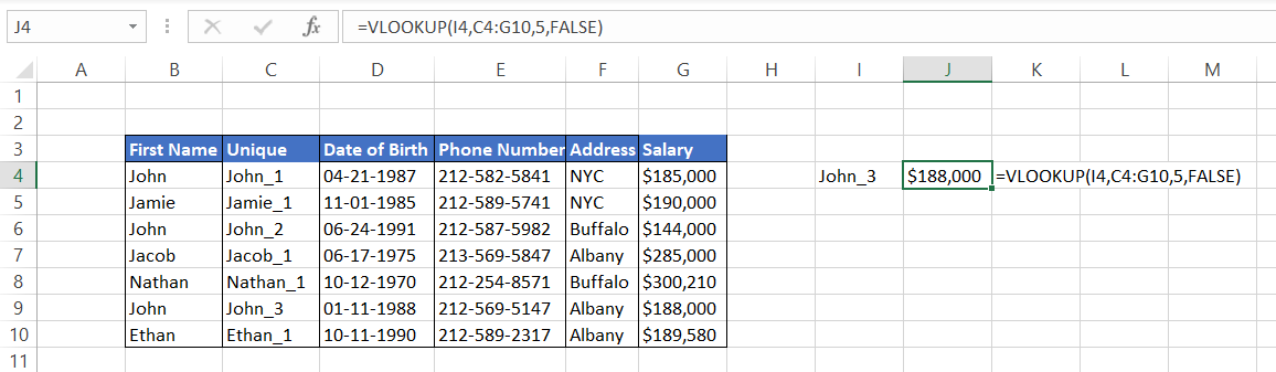
- Matches first value in case of duplicates: Suppose that you need to find the salary for 'John' from your employee database who lives in Buffalo. There is another John who lives in New York City.
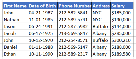
By using the first name as ourlookup_value, enter the formula=VLOOKUP(H5,B4:F10,5,FALSE)in I5. This gives us the value of $185,000. However, on closer inspection, we check that the results retrieved are actually wrong. Even after referencing the correct first name, the formula matches the result for the first value. Now, this is a small dataset. Do you think you can manually check spreadsheets containing hundreds and thousands of rows filled with data?
(Don't worry! We have got a bonus section on how to deal with duplicates later in this article) - Static references: If you insert or delete columns, you might get #REF! error as a result of references becoming invalid. In such cases, you need to edit the formula again to make valid references again.
- 较慢的计算: When you use the 'exact match mode' on big data, it can cause Excel to slow down as it needs to iterate through every single cell of thetable_arrayto find an exact match.
- It is not case-sensitive: When you want to retrieve a value, VLOOKUP treats 'abc' and 'ABC' as the samelookup_value, meaning it does not distinguish between them. This brings limitations in the usage of VLOOKUP on larger data sets.

 However, on closer inspection, we check that the results retrieved are actually wrong. Even after referencing the correct first name, the formula matches the result for the first value. Now, this is a small dataset. Do you think you can manually check spreadsheets containing hundreds and thousands of rows filled with data?
Dealing with duplicates while using VLOOKUP
As an analyst, you will always come across datasets that consist of a significant number of duplicates. Since VLOOKUP will always give you the first value in case of duplicates, it is necessary to have some uniqueness in yourlookup_value. There you have it! That's your solution to the duplicate values - unique identity. For example, suppose you have the below employee database consisting of three different 'John.'

To retrieve the salary for the 'John' in the second-last position, we will be creating unique identities for First Name by using the formula=B4&"_"&COUNTIF($B$4:B4,B4)in cell C4 and dragging it down till the end of the table. This is a combination of CONCATENATE and COUNTIF formula, which will add a column in your table as:

现在,您可以使用vlookup功能在桌上找到不同约翰的工资。但是,请注意,现在我们lookup_valuechanges from B4:B10 to C4:C10, and the table array becomes C4:G10. Including the B column in your formula will give you the #N/A error.
Things to remember about the VLOOKUP Function
vlookupis a versatile function that lets you look up data based on the value of an item in another cell. You can use it to combine information from two tables or to search for something in one table based on some other criteria.
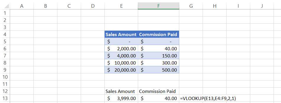
One of the most important things to remember about VLOOKUP is that it's always looking for an approximate match, i.e., therange_lookup参数始终设置为true。因此,如果您正在寻找确切的匹配,则必须将参数设置为false或0。
For example, if you were using VLOOKUP to find how much commission will be paid based on the sales made by the marketing team, then we will use the formula= vlookup(e13,e4:f9,2,1)where therange_lookupis set as TRUE. Even when the sales amount is $3,999, it does not add the commissions applicable on sales of $4,000. In this case, if we had used an exact match, we would have received the #N/A error.
More on Excel
To continue your journey towards becoming an2ManBetX登陆 向导,看看这些额外的有用的堵水resources.


or Want toSign upwith your social account?